Deep neural networks are some of the most powerful learning algorithms that have ever been developed. Unfortunately, they are also some of the most complex. The hierarchical non-linear transformations that neural networks apply to data can be nearly impossible to understand. This problem is exacerbated by the non-determinism of neural network training regimes. Very often small changes in the hyperparameters of a network can dramatically affect the network’s ability to learn.
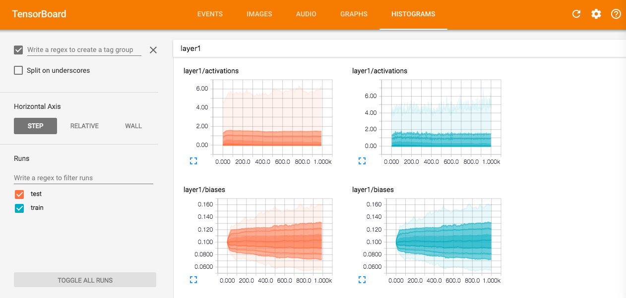
In order to combat this problem, deep learning researchers use a wide array of tools and techniques for monitoring a neural network’s learning process. Even just visualizing a histogram of each layer’s weight matrix or gradient can help researchers spot problems.
After training a network, it’s often helpful for researchers to try to understand how it forms predictions. For example, in this paper researchers use a technique for visualizing how each layer in a convolutional neural network processes an input image by essentially reversing the hierarchical image encoding process.
One question that researchers often ask when evaluating a machine learning model’s prediction on some input is “what features were most important in forming this prediction?” One way to answer this question is to see how the model’s prediction changes when we occlude different parts of the image. Lets say we have a model that is trained to recognize a large number of image classes, including “cat,” and we feed it this image:

If the model is well trained, then it will predict “cat.” But why is it making that prediction? Has it learned to recognize the shape of the cat, or is it just using the litter box next to it as a context clue? We can test this by feeding the model the following images:


If the model generates the correct prediction for the first image and the incorrect prediction for the second image, then we can assume that the model was relying more heavily on the cat’s shape than the context cues in forming its original prediction. But if the model generates the correct prediction in both cases, then we still don’t know the relative weights that the model is placing on the context cues in forming its prediction.
Layerwise Relevance Propagation
Layerwise Relevance Propagation (LRP) is a technique for determining which features in a particular input vector contribute most strongly to a neural network’s output. The technique was originally described in this paper.
The goal of LRP is to define some relevance measure R over the input vector such that we can express the network output as the sum of the values of R:
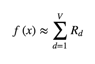
Where \(f\) is the neural network forward pass function. For example, in the case where the input to the network is a natural image, we are decomposing the output of the network into the sum of the relevances of the pixels in the input image. In order to perform this decomposition, we begin with the “relevance” being concentrated at the output node in the graph, and then iteratively “propagate” it backwards through the network.
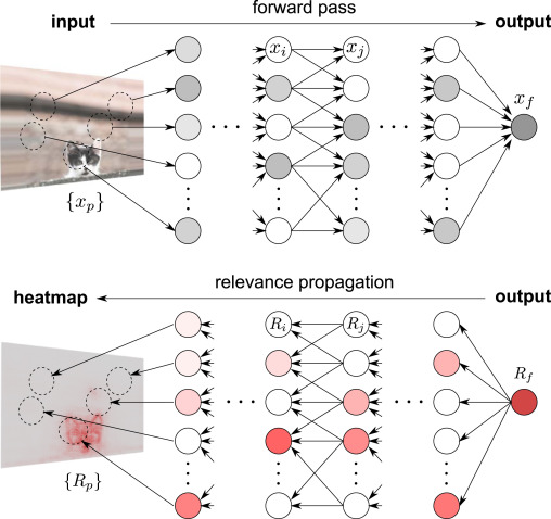
At each layer, the total relevance value is preserved, and the final propagation maps the relevance back onto the input vector. This process is similar in spirit to backpropagation.
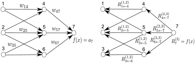
When we perform the propagation procedure, we need to determine how to map the relevance back from some neuron \(n\) at layer \(k\) to the set of neurons \(n_i\) at layer \(k-1\) who feed into neuron \(n\). That is, we need to define a vector valued function that takes in the relevance \(R\) at neuron \(n\), the activation \(x\) of neuron \(n\), the activations \(x_i\) of the neurons \(n_i\) at layer \(k-1\), and the weight matrix \(w\) that connects the neurons \(n_i\) to \(n\), and outputs the relevance of each neuron \(n_i\). Ideally this function will assign higher weights to neurons that had a larger role in influencing the value of \(n\). The original LRP paper defines a set of constraints from which we can derive a number of different relevance propagation functions, but in this post I’m going to focus on the deep taylor decomposition.
Deep Taylor Decomposition
Let’s consider the scalar valued forward propagation function that maps from the layer \(k-1\) activations \(x_i\) to node \(n\)’s activation \(x\). The \(i^{th}\) partial derivative of this function measures the strength of the relationship between \(n_i\)’s activation \(x_i\) and \(n\)’s activation \(x\). So if we can decompose this function in terms of its partial derivatives, we can use that decomposition to approximate the relevance propagation function. Luckily, we can do exactly this with a Taylor Series.
Remember that we can use a Taylor series to approximate the value of a function \(f\) near a point \(x_0\) with:
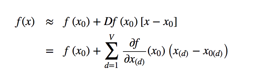
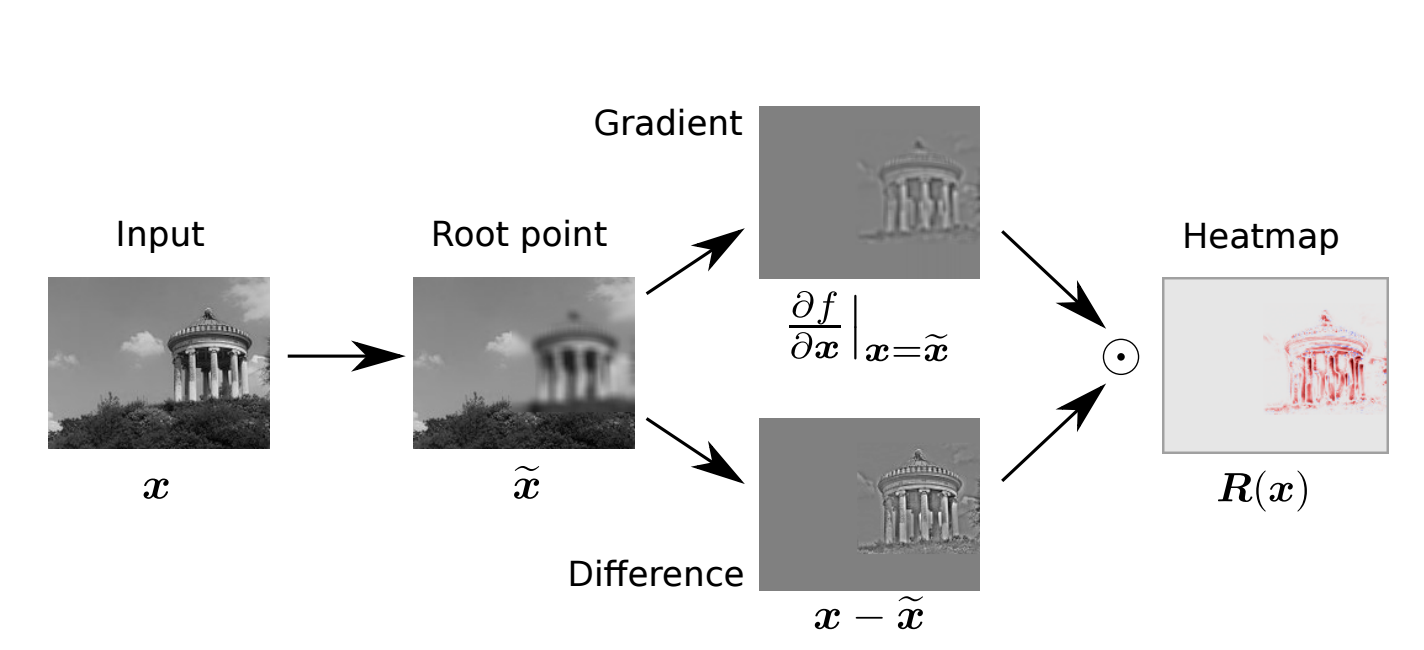
The closer that \(x\) is to \(x_0\), the better the approximation. One clever thing that we can do is set \(x_0\) to be a “root point” of the forward propagation function, that is, a point such that \(f(x_0) = 0\). This simplifies the above Taylor expression to:
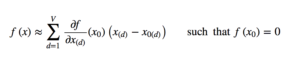
Root points of the forward propagation function are located at the local decision boundary, so the gradients along that boundary point give us the most information about how the function separates the input by class.
LRP Results
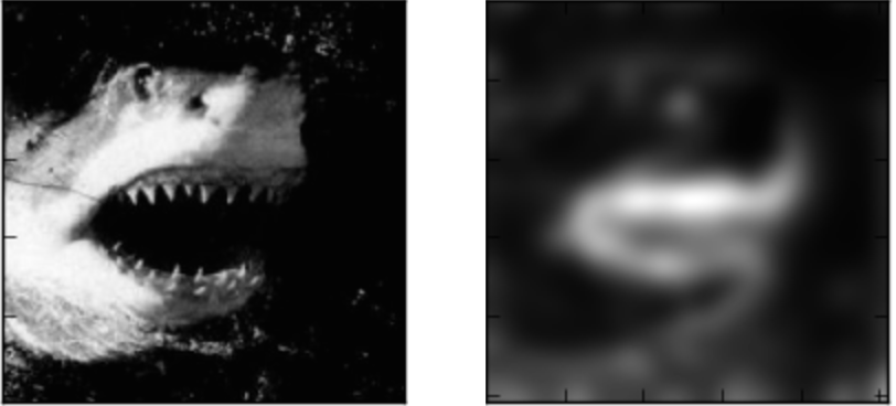
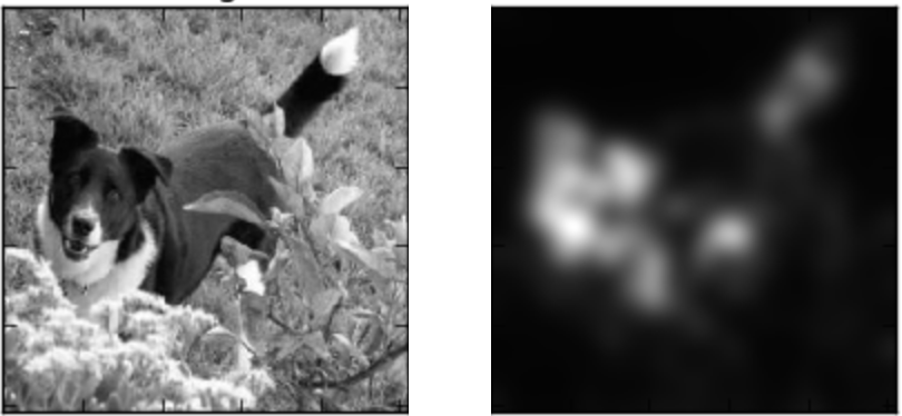
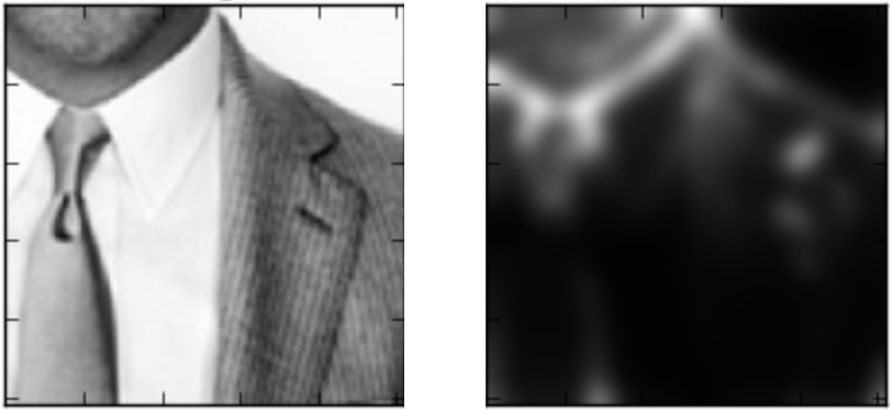
LRP can produce some really helpful and nice-looking visualizations of how a neural network interprets an image.
Here’s how the VGG network interprets a few images:

I implemented a simple TensorFlow-based LRP here. If you’re interested in using it in your research, feel free to send me an email at [email protected].
Conclusion and Further Reading
Layerwise Relevance Propagation is just one of many techniques to help us better understand machine learning algorithms. As machine learning algorithms become more complex and more powerful, we will need more techniques like LRP in order to continue to understand and improve them.
If you’d like to learn more about LRP and Deep Taylor Decompositions, I would highly recommend checking out this website as well as the original LRP paper and this Deep Taylor Decomposition Paper.